Music Genre Classification using Hidden Markov Models
Music genre classification has been an interesting problem in the field of Music Information Retrieval (MIR). In this tutorial, We will try to classify music genre using hidden Markov models which are very good at modeling time series data. As Music audio files are time series signals, we expect that HMMs will suit our needs and give us an accurate classification. An HMM is a model that represents probability distributions over sequences of observations. We assume that the outputs are generated by hidden states. To learn more about HMM click click here. Also, you can find a good explanation for HHMs in the time series use case here.
Dataset & Features
We will use a dataset provided by Marsyas (Music Analysis, Retrieval, and Synthesis for Audio Signals) which is an open source software, called GTZAN. It’s a collection of 1000 audio tracks each 30 seconds long. There are 10 genres represented, each containing 100 tracks. All the tracks are 22050Hz Mono 16-bit audio files in .au format. In our tutorial, we will use all provided genres (blues, classical, jazz, country, pop, rock, metal, disco, hip-hop, reggae). For music genre classification, we will be easier for us to use WAV files, because they can be easily read by the scipy library. We would, therefore, have to convert our AU files to WAV format. The dataset can be accessed here.
For audio processing, we needed to find a way to concisely represent song waveforms. Mel Frequency Cepstral Coefficients (MFCC) is a good way to do this. MFCC takes the power spectrum of a signal and then uses a combination of filter banks and discrete cosine transform to extract features. More details about MFCC can be found here.
Let’s get started by importing the necessary libraries for our project.
1
2
3
4
5
6
7
8
    from python_speech_features import mfcc, logfbank
    from scipy.io import wavfile
    import numpy as np
    import matplotlib.pyplot as plt
    from hmmlearn import hmm
    from sklearn.metrics import confusion_matrix
    import itertools
    import os
Let’s pick one song from our dataset and extract MFCC and Filter banks features.
1
2
3
    sampling_freq, audio = wavfile.read("genres/blues/blues.00000.wav")
    mfcc_features = mfcc(audio, sampling_freq)
    filterbank_features = logfbank(audio, sampling_freq)
We take a look at the shapes of the extracted features.
1
2
3
4
print ('\nMFCC:\nNumber of windows =', mfcc_features.shape[0])
print ('Length of each feature =', mfcc_features.shape[1])
print ('\nFilter bank:\nNumber of windows =', filterbank_features.shape[0])
print ('Length of each feature =', filterbank_features.shape[1])
MFCC: Number of windows = 1496 Length of each feature = 13 Filter bank: Number of windows = 1496 Length of each feature = 26
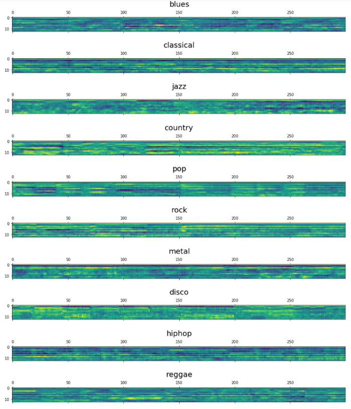
Now, let’s go through some samples of our dataset. We loop over the genres folders and visualize the MFCC features for the first song in each folder.
1
2
3
4
5
6
7
8
9
10
11
12
13
14
15
16
17
import glob
import os.path as path
genre_list = [“blues”,”classical”, “jazz”, “country”, “pop”, “rock”, “metal”, “disco”, “hiphop”, “reggae”]
print(len(genre_list))
figure = plt.figure(figsize=(20,3))
for idx ,genre in enumerate(genre_list):
   example_data_path = ‘genres/’ + genre
   file_paths = glob.glob(path.join(example_data_path, ‘*.wav’))
   sampling_freq, audio = wavfile.read(file_paths[0])
   mfcc_features = mfcc(audio, sampling_freq, nfft=1024)
   print(file_paths[0], mfcc_features.shape[0])
   plt.yscale(‘linear’)
   plt.matshow((mfcc_features.T)[:,:300])
   plt.text(150, -10, genre, horizontalalignment=’center’, fontsize=20)

plt.yscale(‘linear’)
plt.show()
Building Hidden Markov Models
We built a class to handle HMM training and prediction by wrapping the model provided by hmmlearn library.
1
2
3
4
5
6
7
8
9
10
11
12
13
14
15
16
17
18
    class HMMTrainer(object):
    def __init__(self, model_name='GaussianHMM', n_components=4, cov_type='diag', n_iter=1000):
        self.model_name = model_name
        self.n_components = n_components
        self.cov_type = cov_type
        self.n_iter = n_iter
        self.models = []
        if self.model_name == 'GaussianHMM':
        self.model = hmm.GaussianHMM(n_components=self.n_components,        covariance_type=self.cov_type,n_iter=self.n_iter)
        else:
        raise TypeError('Invalid model type')

    def train(self, X):
        np.seterr(all='ignore')
        self.models.append(self.model.fit(X))
        # Run the model on input data
    def get_score(self, input_data):
        return self.model.score(input_data)
Training & evaluating the Hidden Markov Models
For training the Hidden Markov Models, We loop over the subfolder in our dataset, we iterate over the songs in the subfolder in order to extract the features and append it to a variable. We should store all trained HMM models, so we will be able to predict the class of unseen songs. As HMM is a generative model for unsupervised learning, we don’t need labels to build HMM models for each class. We explicitly assume that separate HMM models will be built for each class. Note that we have used 4 as the number of components which is exactly the number of hidden state in the HMM models. Finding out the best number of states is about testing and experimenting with different values and pick the one that optimizes the predictions.
1
2
3
4
5
6
7
8
9
10
11
12
13
14
15
16
17
18
19
20
21
22
23
24
25
26
27
28
29
30
31
32
33
34
    hmm_models = []
    input_folder = 'genres/'
    # Parse the input directory
    for dirname in os.listdir(input_folder):
        # Get the name of the subfolder
        subfolder = os.path.join(input_folder, dirname)
        if not os.path.isdir(subfolder):
            continue
        # Extract the label
        label = subfolder[subfolder.rfind('/') + 1:]
        # Initialize variables
        X = np.array([])
        y_words = []
        # Iterate through the audio files (leaving 1 file for testing in each class)
        for filename in [x for x in os.listdir(subfolder) if x.endswith('.wav')][:-1]:
                # Read the input file
                filepath = os.path.join(subfolder, filename)
                sampling_freq, audio = wavfile.read(filepath)
                # Extract MFCC features
                mfcc_features = mfcc(audio, sampling_freq)
                # Append to the variable X
                if len(X) == 0:
                    X = mfcc_features
                else:
                    X = np.append(X, mfcc_features, axis=0)

                # Append the label
                y_words.append(label)
        print('X.shape =', X.shape)
        # Train and save HMM model
        hmm_trainer = HMMTrainer(n_components=10)
        hmm_trainer.train(X)
        hmm_models.append((hmm_trainer, label))
        hmm_trainer = None
Now it’s time to evaluate our models, We iterate over the test dataset subfolders, we extract the features then we iterate through all HMM models and pick the one with the highest score.
1
2
3
4
5
6
7
8
9
10
11
12
13
14
15
16
17
18
19
20
21
22
23
24
25
input_folder = 'test/'
real_labels = []
pred_labels = []
for dirname in os.listdir(input_folder):

  subfolder = os.path.join(input_folder, dirname)
  if not os.path.isdir(subfolder):
    continue
  # Extract the label
  label_real = subfolder[subfolder.rfind('/') + 1:]

  for filename in [x for x in os.listdir(subfolder) if x.endswith('.wav')][:-1]:
    real_labels.append(label_real)
    filepath = os.path.join(subfolder, filename)
    sampling_freq, audio = wavfile.read(filepath)
    mfcc_features = mfcc(audio, sampling_freq)
    max_score = -9999999999999999999
    output_label = None
    for item in hmm_models:
       hmm_model, label = item
       score = hmm_model.get_score(mfcc_features)
       if score > max_score:
          max_score = score
          output_label = label
pred_labels.append(output_label)
Till now, We have the real label for each song in our test dataset and we have estimated the predicted ones. As our problem is a multiclass classification, the best way to evaluate our model’s performance is to look at the confusion matrix (read more here). We use the confusion matrix provided by sklearn and we visualize it using matplotlib library. First, let’s define a function to take care of the matric plotting. This function prints and plots the confusion matrix. Normalization can be applied by setting normalize=True.
1
2
3
4
5
6
7
8
9
10
11
12
13
14
15
16
17
18
19
20
21
22
23
24
25
26
27
28
29
30
def plot_confusion_matrix(cm, classes,
                          normalize=False,
                          title='Confusion matrix',
                          cmap=plt.cm.Blues):

    if normalize:
        cm = cm.astype('float') / cm.sum(axis=1)[:, np.newaxis]
        print("Normalized confusion matrix")
    else:
        print('Confusion matrix, without normalization')

    print(cm)

    plt.imshow(cm, interpolation='nearest', cmap=cmap)
    plt.title(title)
    plt.colorbar()
    tick_marks = np.arange(len(classes))
    plt.xticks(tick_marks, classes, rotation=45)
    plt.yticks(tick_marks, classes)

    fmt = '.2f' if normalize else 'd'
    thresh = cm.max() / 2.
    for i, j in itertools.product(range(cm.shape[0]), range(cm.shape[1])):
        plt.text(j, i, format(cm[i, j], fmt),
                 horizontalalignment="center",
                 color="white" if cm[i, j] > thresh else "black")

    plt.tight_layout()
    plt.ylabel('True label')
    plt.xlabel('Predicted label')
Time to compute the confusion matrix and visualize it!
1
2
3
4
5
6
7
8
    cm = confusion_matrix(real, pred)
    np.set_printoptions(precision=2)
    classes = ["blues","classical", "country", "disco", "hiphop", "jazz", "metal", "pop", "reggae", "rock"]
    plt.figure()
    plot_confusion_matrix(cm, classes=classes, normalize=True,
                        title='Normalized confusion matrix')

    plt.show()
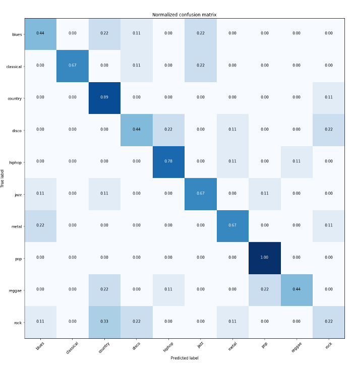
For a perfect classifier, we would have expected a diagonal of dark squares from the left-upper corner to the right lower one, and light colors for the remaining area. As we can see from the matrix plot, The HMM model for the ‘Pop’ class is able to perfectly predict the class of the songs. ‘Country’ and ‘Hip-hop’ are also performing good. However, the worst model is the one for ‘Rock’ class! sorry, rock-fans! For an even better evaluation, It’s always recommended to use the precision and recall metrics for the classification problem. sklearn made it easy for us to have a detailed report about the precision and recall of our multiclass classification. We just need to provide the real and predicted values and our classes names.
1
2
    from sklearn.metrics import classification_report
    print(classification_report(real, pred, target_names=classes))
The output looks like:
1
2
3
4
5
6
7
8
9
10
11
12
13
14
precision    recall  f1-score   support

      blues       0.50      0.44      0.47         9
  classical       1.00      0.67      0.80         9
    country       0.50      0.89      0.64         9
      disco       0.50      0.44      0.47         9
     hiphop       0.70      0.78      0.74         9
       jazz       0.60      0.67      0.63         9
      metal       0.67      0.67      0.67         9
        pop       0.75      1.00      0.86         9
     reggae       0.80      0.44      0.57         9
       rock       0.33      0.22      0.27         9

avg / total       0.64      0.62      0.61        90
Conclusion
That brings us to the end of this tutorial. The performance of our Hidden Markov models is relatively average, and obviously, there is a huge room for improvement. Indeed, the Hidden Markov Models are interpretable and powerful for time series data, however, they require a lot of fine-tuning (number of hidden states, input features …). Next, It would be good to try other approaches for classifying music genres such as a recurrent neural network (LSTM).