Human Activity Recognition using Machine Learning
Human Activity Recognition (HAR) plays an important role in real life applications primarily dealing with human-centric problems like healthcare and eldercare. It has seen a tremendous growth in the last decade playing a major role in the field of pervasive computing. In the recent years, lot of data mining techniques has evolved in analyzing the huge amount of data related to human activity, more specifically, machine learning methods have been been previously employed for recognition include Naive Bayes, SVMs, Threshold-based, Markov chains and deep learning models. Indeed, One important part of the prediction is the selection of suitable models, but also a good selection of relevant features would be benificial in the process of building an accurate model.
In this post, we will try to classify human activity using data captured from embedded inertial sensors, carried by 30 subjects performing activities of daily living. We will extract relevant temporal and spectral features from each signal. Those features are supposed to carry necessary information from each recording.
Tutorial overview
1
2
3
4
5
6
7
8
1. Data preparation
2. Features extraction
    2.1. Temporal feaures
    2.2. Spectral features
    2.3 Feature selection
3. Benchmarking SKlearn models
4. Best model Finetuning
5. Results and conclusion
1. Data preparation
We will be using the publically available dataset called Human Activity Recognition Using Smartphones available in UCI repository. It contains measurements collected from 30 people with age between 19 and 48. The measurements are captured with a smartphone placed on the waist while doing one of the following six activities: walking, walking upstairs, walking downstairs, sitting, standing or laying. The obtained dataset has been randomly partitioned into two sets, where 70% of the volunteers was selected for generating the training data and 30% the test data. The sensor signals (accelerometer and gyroscope) were pre-processed by applying noise filters and then sampled in fixed-width sliding windows of 2.56 sec and 50% overlap (128 readings/window). The sensor acceleration signal, which has gravitational and body motion components, was separated using a Butterworth low-pass filter into body acceleration and gravity. The gravitational force is assumed to have only low frequency components, therefore a filter with 0.3 Hz cutoff frequency was used. From each window, a vector of features was obtained by calculating variables from the time and frequency domain.
The measures are three-axial linear body acceleration, three-axial linear total acceleration and three-axial angular velocity. So per measurement, the total signal consists of nine component.
Fortunately, The dataset is already prepared and splitted into a training and a test sets for us. In reality, most of the time is spent on fetching, preparing, cleaning the data. We will split the test dataset to have some data for validation set to serve the finetuning of our classifers, and keep the test set for final classifiers evaluation.
The following script reads the data, and prepares it as a Numpy array. The script is borrowed from this awesome article.
1
2
3
4
5
6
7
8
9
10
11
12
13
14
15
16
17
18
19
20
21
22
23
24
25
26
27
28
29
30
31
32
33
34
35
36
37
38
39
40
41
42
43
44
45
46
47
48
49
50
51
52
53
54
55
56
57
58
from pathlib import Path
INPUT_FOLDER_TRAIN = Path("UCI HAR Dataset/train/Inertial Signals/")
INPUT_FOLDER_TEST =  Path("UCI HAR Dataset/test/Inertial Signals/")

INPUT_FILES_TRAIN = ['body_acc_x_train.txt', 'body_acc_y_train.txt', 'body_acc_z_train.txt',
                     'body_gyro_x_train.txt', 'body_gyro_y_train.txt', 'body_gyro_z_train.txt',
                     'total_acc_x_train.txt', 'total_acc_y_train.txt', 'total_acc_z_train.txt']

INPUT_FILES_TEST = ['body_acc_x_test.txt', 'body_acc_y_test.txt', 'body_acc_z_test.txt',
                     'body_gyro_x_test.txt', 'body_gyro_y_test.txt', 'body_gyro_z_test.txt',
                     'total_acc_x_test.txt', 'total_acc_y_test.txt', 'total_acc_z_test.txt']

LABELFILE_TRAIN = 'UCI HAR Dataset/train/y_train.txt'
LABELFILE_TEST = 'UCI HAR Dataset/test/y_test.txt'

activities_description = {
    1: 'walking',
    2: 'walking upstairs',
    3: 'walking downstairs',
    4: 'sitting',
    5: 'standing',
    6: 'laying'
}

def read_signals(filepath):
    data = filepath.read_text().splitlines()
    data = map(lambda x: x.rstrip().lstrip().split(), data)
    data = [list(map(float, line)) for line in data]
    return data

def read_labels(filename):
    with open(filename, 'r') as fp:
        activities = fp.read().splitlines()
        activities = list(map(int, activities))
    return pd.Series(activities)

def randomize(dataset, labels):
    permutation = np.random.permutation(labels.shape[0])
    shuffled_dataset = dataset[permutation, :, :]
    shuffled_labels = labels[permutation]
    return shuffled_dataset, shuffled_labels

train_signals =[]
for input_file in INPUT_FILES_TRAIN:
    signal = read_signals(INPUT_FOLDER_TRAIN / input_file)
    train_signals.append(signal)
train_signals = np.transpose(np.array(train_signals), (1, 2, 0))


test_signals = []
for input_file in INPUT_FILES_TEST:
    signal = read_signals(INPUT_FOLDER_TEST / input_file)
    test_signals.append(signal)
test_signals = np.transpose(np.array(test_signals), (1, 2, 0))

train_labels = read_labels(LABELFILE_TRAIN)
test_labels = read_labels(LABELFILE_TEST)
2. Features extraction
Once our data is loaded, we are ready to extract features from it. We will extract two type of features : temporal features which are extracted from the time domain of the signals, and spectral features which are extracted from the frequency domain. We hope that both types carries enough information during our classification task. Most of described and used features are taken from a master thesis that you can enjoy reading here.
2.1 Temporal features
The most obvious way to gain information from a signal is to extract features from its raw representation as a time series. The processed time series can be described throiugh statstical features. Different features describe di erent aspects, so calculating several features from one signal can give comprehensive description of that signal. We will use the following time domain related features:

The mean, the standard deviation and RMS are self-explanatory. Skewness, kurtosis and crest factor as well as L, S and I factors describe the shape of distribution. Skewness measure the symmetry of the distribution which is symmetric about the mean has a skewness close to zero. Kurtosis measure the weight of tails of the distribution. Normal distribution has a kurtosis value close to three, whereas distributions with smaller tails have larger and flatter distributions have smaller values of kurtosis. Crest factor as well as L, S and I factors all describe in their own way, how much the extreme values di er from the rest of the population.
the following function calculate temporal feature from a time series.
1
2
3
4
5
6
7
8
9
10
11
12
13
14
15
16
17
18
19
20
21
22
23
24
25
26
def time_features(series, component=''):
    expected_value = np.mean(series)
    standard_deviation = np.std(series)
    square_mean_root = np.mean(np.sqrt(abs(series)))**2
    root_mean_square = np.sqrt(np.mean(series**2))
    peak_value = np.max(series)
    skewness = skew(series)
    kurtosiss = kurtosis(series)
    crest_factor = peak_value / root_mean_square
    l_factor = peak_value / square_mean_root
    s_factor = root_mean_square / expected_value
    i_factor = peak_value / expected_value

    return {
    'expected_value_'+component : expected_value,
    'standard_deviation_'+component : standard_deviation,
    'square_mean_root_'+component : square_mean_root,
    'root_mean_square_'+component : root_mean_square,
    'peak_value_'+component : peak_value,
    'skewness_'+component : skewness,
    'kurtosiss_'+component : kurtosiss,
    'crest_factor_'+component : crest_factor,
    'l_factor_'+component : l_factor,
    's_factor_'+component : s_factor,
    'i_factor_'+component : i_factor,
}
2.2 Spectral features
Spectral features are frequency based features, they are obtained by converting time based signal into frequency domain using Fourier Transform. In our case, we will convert our time series using Power Spectral Density which is simply the magnitude squared of the Fourier Transform of a continuos time and finite power signal. It is the quantity of power for each frequency component. More specifically, We use the Welch’s methods for calculating PSD as it reduces the spectral leakage.
1
2
3
4
5
6
7
from scipy.signal import welch

f_s = 50

def get_psd_values(y_values, f_s):
    f_values, psd_values = welch(y_values, fs=f_s)
    return f_values, psd_values
Some of the used frequency domain features corespond to the time domain feature and they are described in the following picture.
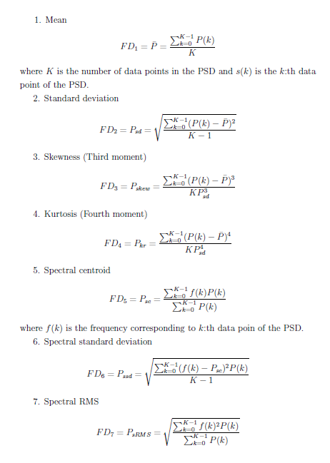
Moreover, we can add other spectral features like spectral flatness, spectral rolloff which determines the frequency below which 85% of the spectrum’s energy is located.
All presented features are easy to calculate with python, the following function produces them for a given PSD.
1
2
3
4
5
6
7
8
9
10
11
12
13
14
15
16
17
18
19
20
21
22
23
24
25
26
27
28
29
30
31
32
33
34
35
36
37
38
39
from scipy.stats.mstats import gmean
from scipy.stats import kurtosis, skew

def rolloff(psd,f):
        absSpectrum = abs(psd)
        spectralSum = np.sum(psd)

        rolloffSum = 0
        rolloffIndex = 0
        for i in range(0, len(psd)):
            rolloffSum = rolloffSum + absSpectrum[i]
            if rolloffSum > (0.85 * spectralSum):
                rolloffIndex = i
                break
        frequency = f[rolloffIndex ]
        return frequency

def spectral_features(psd, f, component=''):
    spec_mean = np.mean(psd)
    spec_std = np.std(psd)
    spec_skewness = skew(psd)
    spec_kurtosiss = kurtosis(psd)
    spec_centroid = np.sum(np.multiply(psd, f)) / np.sum(psd)
    spec_std_f = np.sqrt(np.sum(np.multiply((f - spec_centroid)**2,psd)) / (len(psd) - 1))
    spec_rms = np.sqrt((np.sum(np.multiply(f**2,psd))) / (np.sum(psd)))
    spec_flatness = gmean(psd) / np.mean(psd)
    spec_rolloff = rolloff(psd,f)

    return {
        'spec_mean_'+component : spec_mean,
        'spec_std_'+component : spec_std,
        'spec_skewness_'+component : spec_skewness,
        'spec_kurtosiss_'+component : spec_kurtosiss,
        'spec_centroid_'+component : spec_centroid,
        'spec_std_f'+component : spec_std_f,
        'spec_rms_'+component : spec_rms,
        'spec_flatness_'+component : spec_flatness,
        'spec_rolloff_'+component : spec_rolloff,
    }
For each time series in our datasets, the process of extracting all features, temporal and spectral, will result of 21 feature. In our dataset we have 7352 signal in the training set and 2947 in the test set, each signal with 9 components, which results of 189 features per signal.
Now it’s time to go through our dataset and generate all features and put them in a clean dataframe.
1
2
3
4
5
6
7
8
9
10
11
12
13
14
15
def generate_all_features(signals):
    all_features = []
    for signal in tqdm(signals):
        signal_features = {}
        for i in range(9):
            series = signal[:, i]
            f, psd = get_psd_values(series, f_s)
            signal_features_cpt = {**spectral_features(psd, f, signal_id=str(i)), **time_features(series, signal_id=str(i))}
            signal_features = {**signal_features, **signal_features_cpt}
        all_features.append(signal_features)
    return pd.DataFrame(all_features)

df_train = generate_all_features(train_signals)
df_test = generate_all_features(test_signals)
3. Benchmarking different classifiers
After preparing all the features for the training and test sets, we can now train a classifier to recognize the human activity. We will do a quick benchmark of different available classifier and pick the best one and optimize it further. In addition to XGBoost, our list includes a collection of classifier from the amazing library scikit-learn.
This script instanciate different classifiers and train them using training data and calculate their score on test set.
1
2
3
4
5
6
7
8
9
10
11
12
13
14
15
16
17
18
19
20
21
22
23
24
25
26
27
28
29

def benchmark(clf, clf_descr):
    t0 = time()
    clf.fit(df_train, train_labels)
    train_time = time() - t0
    t0 = time()
    pred = clf.predict(df_test)
    test_time = time() - t0
    score = accuracy_score(test_labels, pred)
    return clf_descr, score, train_time, test_time


models = [(RidgeClassifier(tol=1e-2, solver="lsqr"), "Ridge Classifier"),
        (MLPClassifier(alpha=1, max_iter=50), "MLP"),
        (PassiveAggressiveClassifier(n_iter=50), "Passive-Aggressive"),
        (KNeighborsClassifier(n_neighbors=10), "kNN"),
        (xgb.XGBClassifier(n_estimators=100), "XGBoost"),
        (SGDClassifier(alpha=.0001, n_iter=50, penalty="elasticnet"), 'SGD Classifier'),
        (NearestCentroid(), 'Nearest Centroid - Rocchio' )]


for penalty in ["l2", "l1"]:
    models.append((LinearSVC(penalty=penalty, dual=False,tol=1e-3), f'Linear SVC {penalty}'))
    models.append((SGDClassifier(alpha=.0001, n_iter=50,penalty=penalty), f'SGD Classifier {penalty}'))


results_all = []
for clf, name in tqdm(models):
    results_all.append(benchmark(clf, name))
Once models are trained, we can plot their scores and training time, I have also trained the proposed models using temporal and spectral features to se which set of features could perform better.
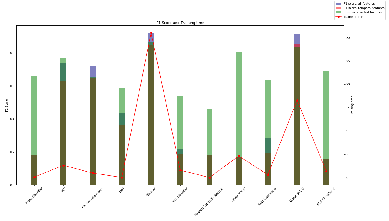
As it’s expected the ensemble model perform better in this classification task. XGBoost has the highest score, but it took the longest to train.
4. Best model Finetuning : XGBoost tuning with HyperOpt
XGBoost has a large number of advanced parameters, which can all affect the quality and speed of our classifier, by quality we mean a model that avoid overfitting and generalize well. To achieve that, we can control model complexity by tweaking max_depth, min_child_weight and gamm parameters, or adding randomness to make training robust to noise with subsample and colsample_bytree. You can read more about XGBoost finetuning here.
In our case, we will use HyperOpt, a Python library for serial and parallel optimization over search spaces, which may include real-valued, discrete, and conditional dimensions. It allows for simple applications of Bayesian optimization. For more details about this topic, check this detailed post.
The following code defines our parameter search space, an objective function to minimize and trails to store the history of our search.
1
2
3
4
5
6
7
8
9
10
11
12
13
14
15
16
17
18
19
20
21
22
23
24
25
26
27
28
29
30
31
32
33
34
35
36
37
38
39
40
from hyperopt import hp, tpe, STATUS_OK, Trials
from sklearn.metrics import mean_absolute_error, log_loss, f1_score
from hyperopt.fmin import fmin

space ={
        'n_estimators': hp.quniform('n_estimators', 500, 100, 100),
        'learning_rate' : hp.loguniform('learning_rate', -6.9, -2.3),
        'max_depth': hp.choice('max_depth', np.arange(10, 30, dtype=int)),
        'min_child_weight': hp.quniform ('min_child', 1, 20, 1),
        'alpha'       : hp.uniform('alpha', 1e-4, 1e-6 ),
        'gamma'      : hp.uniform('gamma ', 1e-4, 1e-6 ),
        'subsample': hp.uniform ('subsample', 0.8, 1)
    }

def objective(space):

    clf = xgb.XGBClassifier(n_estimators = int(space['n_estimators']),
                            max_depth = space['max_depth'],
                            learning_rate = space['learning_rate'],
                            alpha = space['alpha'],
                            gamma  = space['gamma'],
                            min_child_weight = space['min_child_weight'],
                            subsample = space['subsample']
                           )

    eval_set  = [( df_train, train_labels), ( X_validation, y_validation)]

    clf.fit(df_train, train_labels, eval_set=eval_set, eval_metric="mlogloss", verbose=False)

    pred = clf.predict_proba(X_validation)
    mlogloss = log_loss(y_validation, pred)
    print('Loss', mlogloss)
    return{'loss':mlogloss, 'status': STATUS_OK }

trials = Trials()
best = fmin(fn=objective,
            space=space,
            algo=tpe.suggest,
            max_evals=20,
            trials=trials)
After finishing the space search for optimal parameters, the best set of paramaters are returned and used to train the best version of our classifier, we provide an evaluation set to track the progress of our model’s learning. Then, we can plot the classification error and the loss in our predictions.
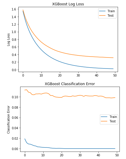
It seems like out model stopped learning after iteration 20, Thus, It would be better to have an early stoping around 20. One of the advantages of XGBoost is its interpretability through features importance. We can see what are the most useful features for performing predictions on the leaf nodes of our models’ estimators.
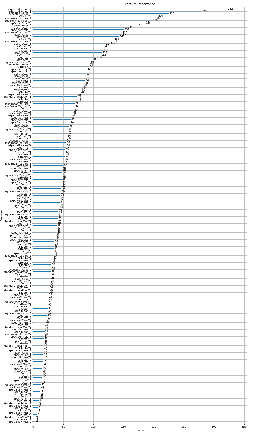
The last three component of our signal seem to have most relevant information when classifying humain activity. Now let’s look how our model did with respect to each class in our dataset, this can be summarized in the classification report provided by scikit-learn.
1
2
3
4
5
6
7
8
9
10
11
12
              precision    recall  f1-score   support

           1       0.90      0.95      0.92       496
           2       0.92      0.96      0.94       471
           3       0.95      0.86      0.90       420
           4       0.91      0.82      0.86       491
           5       0.85      0.92      0.88       532
           6       1.00      1.00      1.00       537

   micro avg       0.92      0.92      0.92      2947
   macro avg       0.92      0.92      0.92      2947
weighted avg       0.92      0.92      0.92      2947
We can also look at the famous confusion matrix to evaluate the performance of our classifier on the test set.
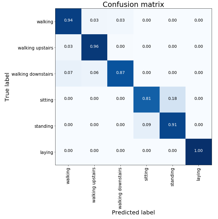
Our classifier is able to recognize human activity with a pretty good accuracy across all activities.
5. Conclusion
That brings us to the end of this tutorial. We have built a classifier for human activity recognition based on temporal and spectral features extracted from signal data coming from human daily activities. We have experimented with a collection of classifiers and we picked the best one which is, as expcted, XGBoost model. Furthermore, we tried to optimize the XGBoost model by performing the hyper-parameter finetuning using HyperOpt to pick the best parameter of our classifier.
For further experiments, we can try using the entier time series signal data instead of extracting features, and use a time series based classifiers like Hidden Markov Models or Ruccurrent Neural network.