Bayesian Optimization
Bayesian Optimization is a useful tool for optimizing an objective function thus helping tuning machine learning models and simulations. Instead of using standard approaches like random search or grid search which are usually expensive or slow to do and where the objective function is a black box (we can not analytically express f or know its derivative), Bayesian Optimization comes in hand to efficiently trades of between exploration and exploitation to find a global optimum is a minimum of number of steps. It mainly rely on the idea of Bayes theorem , posterior = likelihood * prior, to quantify the beliefs about an unknown objective function given samples from the domain \(D\) and their evaluation via the objective function \(f\). Bayesian optimization incorporates prior belief about \(f\) and updates the prior with samples drawn from f to get a posterior that better approximates \(f\). (\(P(f|D) = P(D|f) * P(f)\)).
Furthermore, an other advantage of this method is its ability to be effective in practice in a situations where the underlying function f is stochastic, non-convex or even non-continuous.
Bayesian Optimization using Gaussian Processes.
In order to optimize an objective function, Bayesian Optimization uses fundamentally two main models, a probabilistic regression model called in this context a surrogate model, and a function that samples from areas where it’s most likely to find an improvement comparing to our current observation named an acquisition function.
The Bayesian optimization procedure goes as follows :
For \(t=1,2 ...\):
- Find \(X_t\) by optimizing the acquisition function \(u\) over the function f.
- Sample the objective function : \(f(X_t)\)
- Augment the inputs with the new sample \(\{X_1, X_2, ...X_{t-1},X_t\}\) and update the posterior of function \(f\) using the surrogate model.
Surrogate models : Gaussian Processes
Surrogate models are used in the context of Bayesian optimization due to their ability of defining a predictive distribution that captures the uncertainty in the surrogate reconstruction of the objective function. Some of those model that are worth mentioning are : Gaussian Processes, Random Forrest, and Tree Parzan Estimators. In practice, Gaussian Processes have become a popular and widely used surrogate model for modeling objective function in Bayesian optimization. they allow us to infer a function simply from its inputs and outputs, and also provide a distribution over the outputs.
Gaussian Process is a technique built on the basis of Gaussian stochastic process and Bayesian learning theory. Contrary to what we usually do in supervised learning situations where we infer a distribution over parameters of a parametric function, Gaussian process can be used to infer a distribution over functions and govern their properties. Based on the assumption that similar input produce similar outputs, Gaussian processes assume a statistical model of a function f that maps \(\{X_1, X_2, ... , X_t\}\) to \(\{f(X_1), ..., f(X_n)\}\), when those mappings are unknown, and in Bayesian statistics, we assume that their are drawn by nature from a prior probability distribution. This prior distribution is set to be a multivariate normal distribution defined by a mean function \(m : X \to R\) and its covariance function or kernel \(K : X \times X \to R\). We denote PG as :
\(f(X) \sim GP(m(X) , K(X,X'))\).
We construct the mean vector by evaluating a mean function m at each xi. We construct the covariance matrix by evaluating a covariance function or kernel k at each pair of points \(\)X_i\(\), \(X_j\) . The kernel is chosen in a way that points closer in the input space are more strongly correlated and kernels are required to be positive semi-defined functions. The most popular Gaussian mean function is a constant value, \(m(X) = \mu\). Usually for the sake of notation simplicity, we assume that it’s equal to zero. but when we know that the function f has a trend or some specific parameter structure, we may take the mean function as \(m(X) = \mu + \sum\limits_{1}^{t} \beta_i \Psi_i(X)\) where each \(\Psi_i\) is a parametric function, and often a low-order polynomial in \(X\).
For covariance function, we have couple of choices, but the mostly used ones are the power exponential (Gaussian) kernel described as follows
\[K(X, X') = \sigma_0 exp(-{1 \over 2l^2} \|{X - X'}\| )\]The length parameter \(l\) controls the smoothness of the function and σf the vertical variation. For simplicity, we use isotropic kernel where all input dimensions have the same length parameter \(l\). An other commonly used kernel is the Matern kernel.
After observing some data \(y = \{f_1, ..., f_t\} = \{f(X_1), ..., f(X_t)\}\)
we can convert GP prior \(p(f/X=\{X_1, X_2, ... , X_t\})\) into a GP posterior \(p(f/X,y)\) assuming that the function values \(f\) are drawn according to multivariate normal distribution \(N(0, K)\) where
\[K = \begin{bmatrix}k(X_1,X_1) & k(X_1,X_2) & .&.&. & k(X_1,X_t) \\ k(X_2,X_1) & k(X_2,X_2) & .&.&. & k(X_2,X_t) \\ .\\.\\ k(X_t,X_1) & k(X_t,X_2) & .&.&. & k(X_t,X_t) \end{bmatrix}\]Each element in \(K\) represents the degree of approximation between two samples. Thus, the diagonal element \(K(X_i, X_i)=1\) if we don’t consider the effect of noise.
Based on the assumption of Gaussian process, if \(f(X_{t+1})\) = \(f_{t+1}\) for a new sample \(X_{t+1}\) then \(\{f_1, ..., f_t, f_{t+1}\}\) follows a \(t+1\) dimensional normal distribution :
\(\begin{bmatrix} f_1 \\ .\\.\\ f_t \\ f_{t+1} \end{bmatrix} \sim N(0, \begin{bmatrix} K & k \\ k^T & K(X_{t+1}, X_{t+1})\end{bmatrix} )\) , where \(k = [K(X_{t+1}, X_1) K(X_{t+1}, X_2) ... K(X_{t+1}, X_t)]\)
The function \(f_{t+1}\) follows 1-dimensional normal distribution \(f_{t+1} \sim N(\mu_{t+1}, \sigma_{t+1}^2)\). by the properties of joint Gaussian we have :
\[\mu_{t+1}(X_{t+1}) = k^T K^{-1}\begin{bmatrix} f_1 &...& f_t\end{bmatrix}\] \[\sigma_{t+1}^2(X_{t+1}) = -k^TK^{-1} + K(X_{t+1},X_{t+1})\]The above equations return the probability distribution over all possible values of \(f_{t+1}\).
Acquisition Function
Bayesian optimization uses the acquisition function \(u\) to derive the maximum of the function \(f\). With the assumption that the maximum value of the acquisition function \(u\) corresponds the maximum value of the objective function \(f\), the acquisition function does a trade off between exploitation and exploration.
\[X_t=argmax_x u(X|\{X_n , f(X_n)\}_{n=1}^{t-1})\]There are couple of popular acquisition functions like Probability of improvement, Expected improvement (EI) and ) GP upper confidence bound (GP-UCB).
Expected improvement (EI)
The function Expected Improvement evaluate the expectation of the degree of improvement that a point can achieve when exploring the area near the current maximum value. Let \(f_t^* = max_{(m<=t)} f(X_m)\) be this maximum value, where \(t\) is the number of times we have evaluated \(f\) thus far. Suppose now that we can have an additional evaluation to perform at \(x\), the new best observed point will either be \(f(x)\) if \(f(x) \geq f_t^*\) or \(f_t^*\) if \(f(x) \leq f_t^*\). The improvement in the new best observed point is then \(max([f(x) - f_t^*],0)\).
As we don’t know \(f(x)\) until after the evaluation and we would like to pick \(x\) where the before mentioned improvement is large, we can take the expected value of this improvement and choose \(x\) that maximize it. Thus, we define the expected improvement as :
\[I(X) = max([f_{t+1}(X) - f_t^*,0]\] \[EI_{t+1}(X_{t+1}) = E[I(X_{t+1})]\] \[X_{t+1} = argmax E_t[I(X_{t+1})]\]When \(f_{t+1}(X) - f_t^* \geq 0\) , the distribution \(f_{t+1}(X)\) follows a normal distribution with the mean \(\mu_{t+1}\) and the standard deviation \(\sigma_{t+1}^2\), thus, the random variable \(I\) follows the normal distribution with the mean \(\mu_{t+1} - f_t^*\) and the standard deviation \(\sigma_{t+1}^2\) .
The expected improvement can be evaluated analytically under the GP model
\[EI_{t+1}(X_{t+1}) = \int_{I=\infty} ^ {I=\infty} f(I) \, dI = \int_{I=0} ^ {I=\infty} I {1 \over {\sqrt{2\pi} \sigma_{t+1}(X_{t+1})} } \exp{-{\mu_{t+1}(X_{t+1}) - f_t^* - I \over {2\sigma_{t+1}^2(X_{t+1})} }} \, dI\] \[EI_{t+1}(X) = \sigma_{t+1}(X) [Z\Phi(Z) + \varphi(Z) ]\]where \(Z = { { \mu_{t+1}(X) - f_t^* - \xi} \over {\sigma_{t+1}(X)}}\) and \(\mu_{t+1}, \sigma_{t+1}\) are, respectively, the mean and the standard deviation of the Gaussian Process posterior. \(\Phi\) and \(\varphi\) are cumulative distribution function (CDF) and probability density function (PDF) respectively. \(\xi\) the amount of exploration during optimization and it’s recommended to have a default value of 0.01.
Probability of improvement (PI)
Probability of improvement explores area near the current optimal value in order to find the points most likely to prevail over the current optimal value. Only when the difference between the value of the next sampling point and the current optimal value is greater than $\xi$, the new sampling point replaces the current optimal value. In this way we try to prevent the situation where the sampling point is limited in a small range and easy to fall into the local optimal solution. The extended PI function expression is defined as :
\[PI_{t+1}(X) = P(f(X) \leq f_t^* + \xi) = \Phi(Z)\]GP upper confidence bound (GP-UCB)
The function GP-UCB determines whether the next sampling point should make use of the current optimum value or should explore other low confidence zone. The parameter \(\beta\) is a hyper-parameter to tune the exploration-exploitation balance. If \(\beta\) is large, it emphasizes the variance of the unexplored solution (i.e. larger curiosity). The definition of the function is defined as :
\[UCB_{t+1}(X) = \mu_{t+1}(X) + \beta \sigma_{t+1}(X)\]An Example
We consider the following function :
\[f(X) = \sin({2 \pi X}) + X^2 + 0.5X + \exp({-X^2 \over 10}) + {1 \over X^2 + 1}\]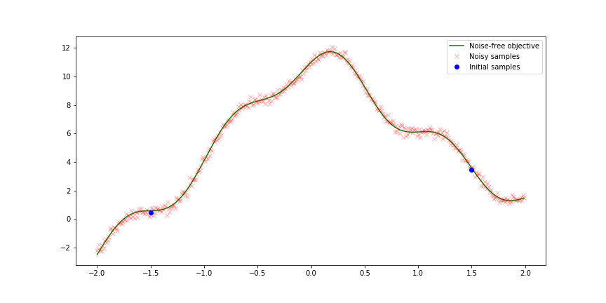
We will treat it as black box and approximate it using Bayesian Optimization. We assume that we have two initial samples. The main goal is find the global optimum in few number of steps. The following picture show the result of Bayesian optimization using different acquisition function we presented previously.
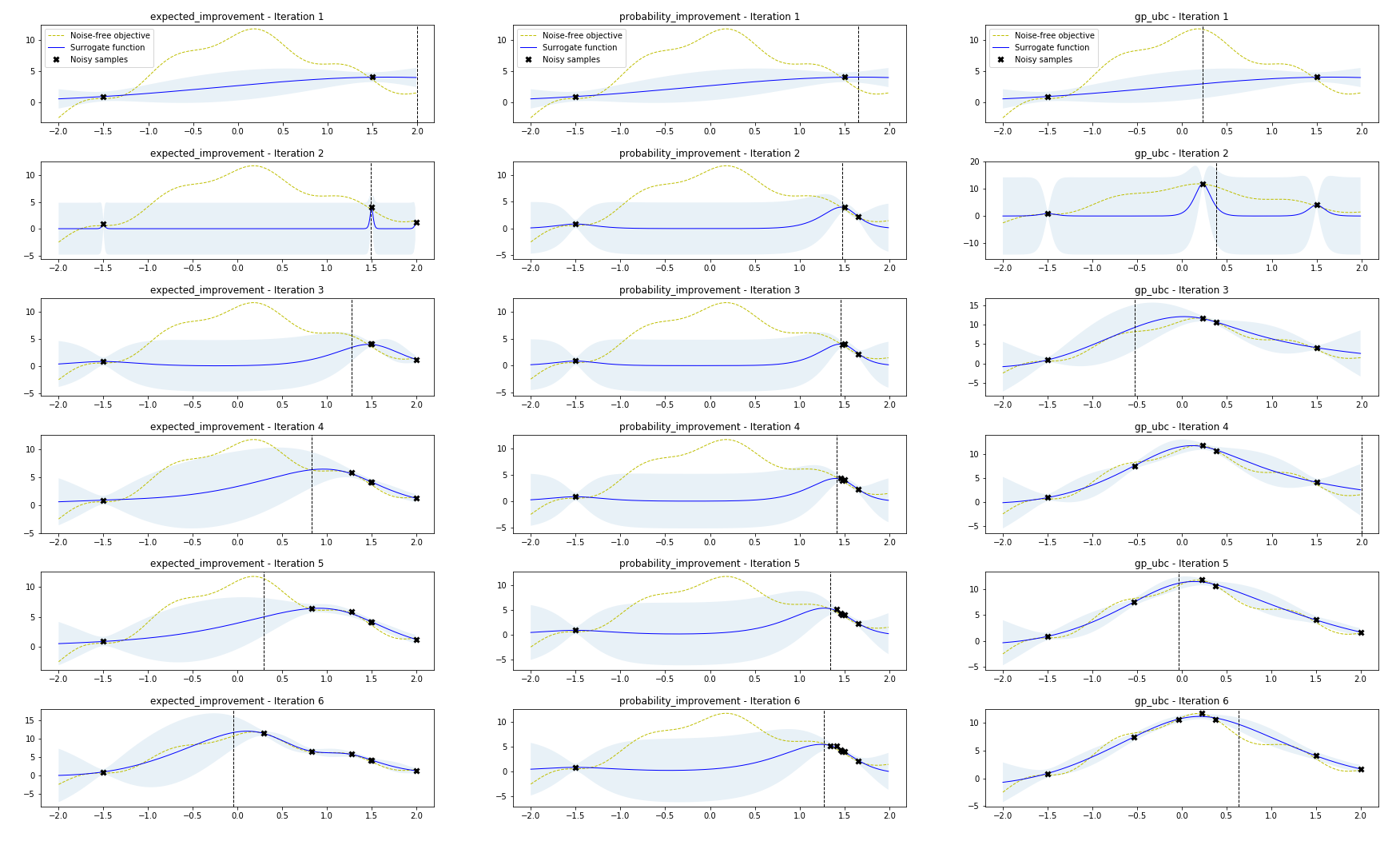
In order to determoine the best acquisition function in our case, we compared the three acquisition functions with the same Gaussian process posterior while optimizing the same function. As we can see, after 10 iterations, the EI and GP-UCB are capable of finding the global optimum solution, while PI function got stuck in the local optimum value.
We can also notice how EI and GP-UCB strategy balances between exploration and exploitation. they sample from regions with high uncertainty (exploration) rather than considering the values where the surrogate function is high.
The Bayesian Optimization has been used in to solve wide range of optimization problems including hyperparameters tuning for machine learning algorithms, reinforcement learning, drug discovery …